Neural Reckoning

Welcome to my introduction to quantum computing. Over the course of this post we will go over the most basic of concepts (bits and gates), and end by solving the simplest problem that cannot be solved by a classical computer, using a quantum circuit simulator that you can play with right within your browser. Extra resources and notes on some of the complexities I’ve skipped can be found at the end. Let’s dive in!

What is a quantum bit?

A nice analogy for bits is to think of them as coins being flipped. In a classical computer these coins are very ‘heavy’ and cannot be thrown into the air. The only possible action we can perform is therefore to turn them over, from heads to tails or vice versa (more commonly known as 0 or 1). A quantum bit, however, is light, and can be thrown into the air. While a coin is flipped into the air and spinning, we do not know whether it is going to land on heads or tails. This doesn’t seem very useful at first glance, but our quantum coin has a couple of special properties:

The coin can be biased to land on either heads or tails more often (or always).
We can only look at a coin once it has landed.
A coin’s bias can be manipulated, even as the coin is still spinning in the air.

Let’s unwrap the metaphor by formalising the above list using more common terminology. The bias in property 1 is known as a ‘superposition’ of the states heads and tails. Mathematically, this is simply a pair of numbers, one that represents heads, $h$ , and another that represents tails, $t$ , with the one condition that $h^2+t^2=1$ . Every possible qubit is therefore nicely visualised using a shape with a similar signature: the humble circle.

A circular visualisation of the possible states of a single qubit, with important states labeled with their exact values.

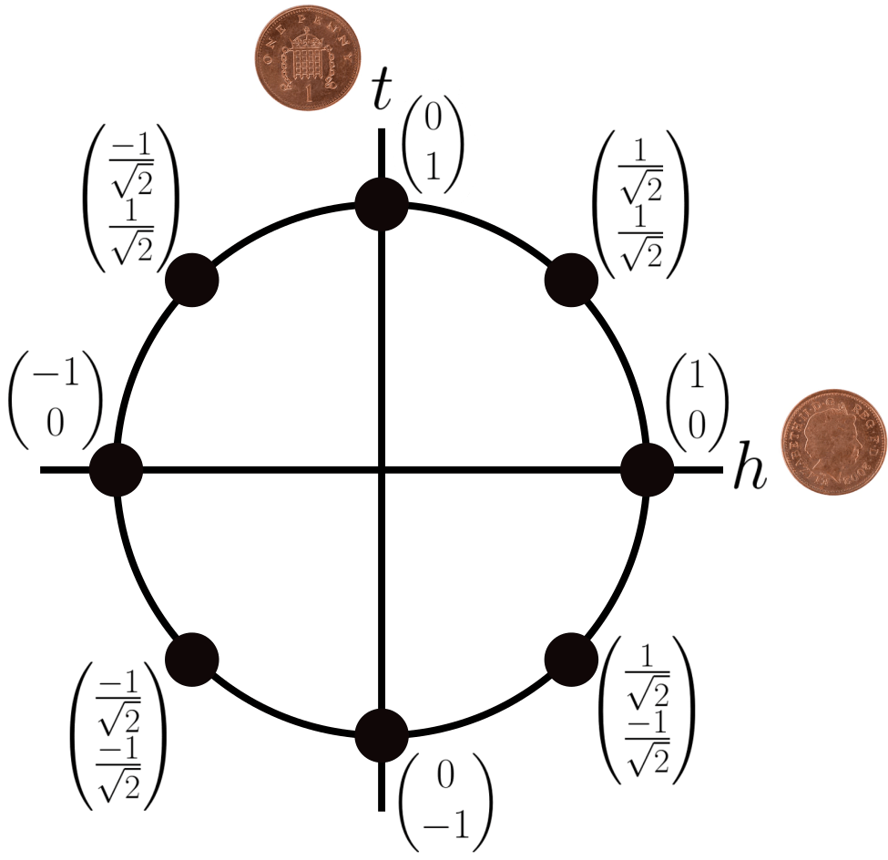
How do these pairs of numbers relate to a biased coin? Through a process known as ‘measurement’ (or sometimes ‘observation’), which is equivalent to the landing of the coin in property 2. When a coin lands, it will be heads with probability $h^2$ and tails with probability $t^2$ . In fact, this means that the 4 states on the diagonal of the circle above will produce the exact same results when measured! Specifically, this is because if we square the individual numbers inside their state, they all produce the same result of $\frac{1}{2}$ for both heads and tails. This is all despite the biases strangely being able to take negative numbers which, spoiler, will actually come in handy for solving our problem at the end of this post.

We will use this representation for all single qubit operations, but be warned that things will get a bit hairy when multiple qubits are involved. You will understand why later, but for now this representation is great for getting a firm grip on manipulating single qubits. But how do we even get a qubit into one of the points on the above circle? This brings us to property 3, for which we need to introduce the concept of quantum gates.

What is a quantum logic gate?

All quantum circuits start with qubits in state $\begin{pmatrix}h\\t\end{pmatrix}=\begin{pmatrix}1\\0\end{pmatrix}$ or $\begin{pmatrix}0\\1\end{pmatrix}$ . To move them into different positions on the edge of the state circle, we need to apply what are known as quantum logic gates.

We will start by learning some single-qubit gates. The first is the Pauli-X gate (sometimes known as a bit-flip, and denoted with an X) which simply switches the biases of heads and tails. The effect of this on our circular visualisation can be seen in the following diagram:

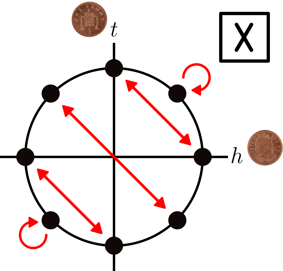
The Pauli-X gate, visualised as a circular state machine.

where the red arrows point to where an application of the gate moves the state of the qubit. As you can see, this gate simply acts as a mirror along the north-eastern diagonal, directly flipping the probabilities of heads and tails. You should also notice that every arrow points in both directions, which means that applying the gate twice brings you back to where you started. The second gate we will use is known as the Hadamard gate (denoted by a H), and it has the following effect:

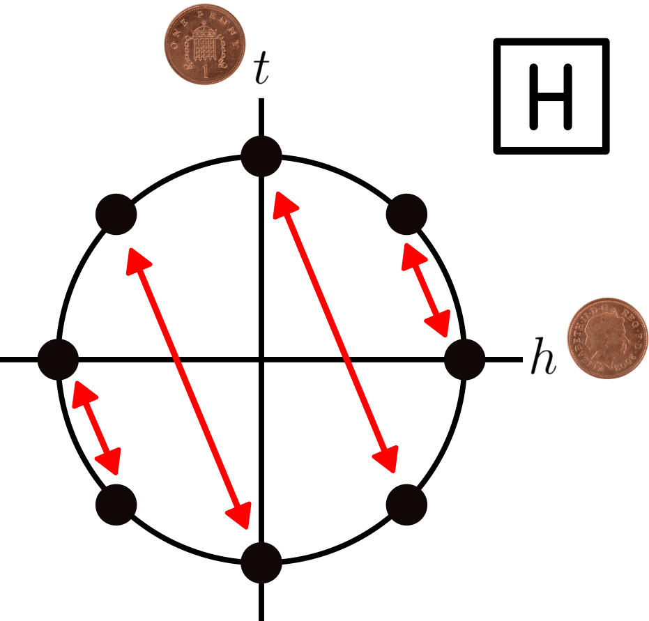
The Hadamard gate, visualised as a circular state machine.

This is similar to the X gate in the sense that it acts as a mirror along a certain axis, which of course also means that applying the gate twice also brings you back to where you started. Starting from any of the 8 positions on the circle, we can now reach any of the other states through a series of gates. For example, if we start at $\begin{pmatrix}1\\0\end{pmatrix}$ , we can get to $\begin{pmatrix}\frac{1}{\sqrt{2}}\\\frac{-1}{\sqrt{2}}\end{pmatrix}$ by applying and X and then a H like this:

See if you can figure out yourself how to get to the state $\begin{pmatrix}-1\\0\end{pmatrix}$ from the same starting point! And note that these 8 qubit values will be the only ones we make use of within this post.

What about multiple qubits?

Dealing with multiple qubits is the same as flipping multiple coins simultaneously. For example, with a single coin we have 2 possible outcomes, heads or tails: $(h,t)$ . With 2 coins, we can have 4 possible outcomes: $(hh,ht,th,hh)$ . With 3 coins, we have 8: $(hhh,hht,hth,htt,thh,tht,tth,ttt)$ . With 4 we have 16, with 5 we have 32 etc. Some of you may have just heard a whisper of exponential speedup, and you would be right: the combination of the biases of multiple coins is in fact exponentially bigger than the number of coins being flipped, and taking advantage of this is key to the power of quantum over classical. However for the purposes of this post we will only need 2 simultaneous coins to solve our target problem.

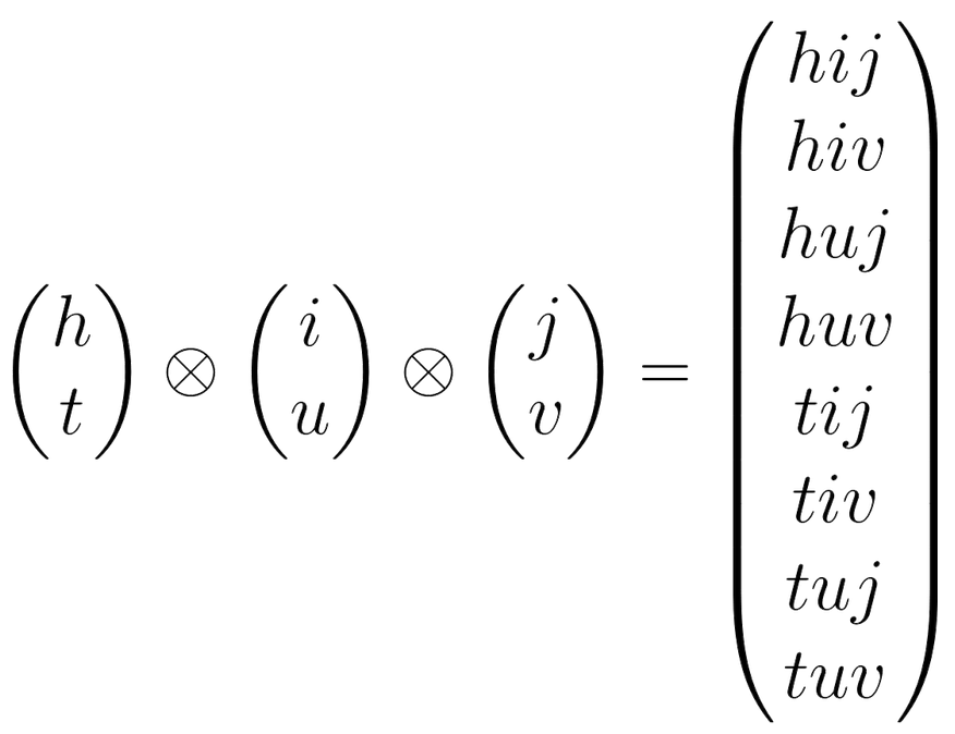
Let us first is to formalise the concept of combining the biases of multiple coins. Unfortunately at this point I do not know of a visualisation as nice as the previous circle state machines, so we will go back to the standard column vector notation (which is good to get used to anyway!). The joint state of multiple coins is expressed with an operation known as the ‘tensor product’, which is something which everyone that has studied GCSE maths has also done before: expanding brackets using the FOIL method. Specifically this looks like:

The tensor product (denoted by a circle with a cross inside) of 2 qubits.

where the resulting quartet of values is known as the superposition of the two inputs. When we measure this superposition it ‘collapses’ back into its 2 individual coins landed as heads or tails, where the probability of each of the 4 combinations of heads and tails is determined by squaring the corresponding terms in the superposition. For example the probability of both coins being heads with the above notation is $(hi)^2$ , while the probability of the first being tails but the second being heads is $(ti)^2$ . Just for fun, with 3 qubits this looks like:

The (monstrous) tensor product of 3 qubits. Note that you can evaluate either of the two tensor products first, and the final result will stay the same. However, swapping the order of qubits themselves will not produce the same result. Also note that the resulting column is fun to read aloud from top to bottom.

which looks big and scary, but don’t worry because we won’t need it for the rest of this post. Going back to 2 qubits, we can now apply one final logic gate, known as the Controlled NOT (or CNOT) gate. Unlike the X and H gates, a CNOT takes the superposition of two qubits as input, and behaves by flipping the last two entries. For example, its behaviour on 4 of the simplest superpositions are:

The effect of a CNOT gate applied to 4 basic superpositions. Try staring for a while to get a sense of the patterns that emerge at each step.

The name Controlled NOT comes from the fact that its effect can be interpreted as the first qubit as controlling whether the second is flipped. When it is set to $\begin{pmatrix}1\\0\end{pmatrix}$ the gate has no effect, but when it is $\begin{pmatrix}0\\1\end{pmatrix}$ the second bit flips, just as if a standard X gate were applied. I personally do not like using this intuition, and prefer to simply think of the 3rd and 4th entries in the superposition being flipped, for a reason that will be made clear once we understand entanglement.

Entanglement

A good question to ask at this point is: why can we not use the previous circular state machine to visualise superpositions of 2 qubits? All of the example inputs to the CNOT gate above should and would work by drawing two separate circles at each step. Where things get a little tricky is in the fourth and final property of our quantum coin:

The biases of simultaneously flipped coins can be manipulated such that they become inextricably linked with each other.

This is perhaps the most important concept I will teach today, but frustratingly is also what breaks our nice circular state machine, as we will see by the end of this section. It is known as ‘entanglement’ (yes, the same entanglement that Einstein himself said was spooky), and I will attempt to explain it through the medium of an interactive quantum circuit simulator! Please try opening it yourself at jxz12.github.io/QuantumVis. When you first start the simulator it should look like this:

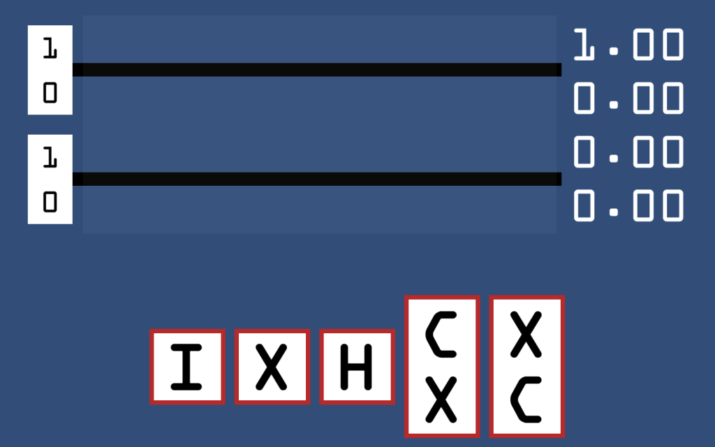
The circuit runs from left to right with 2 input qubits, both of which can be flipped between $\begin{pmatrix}1\\0\end{pmatrix}$ and $\begin{pmatrix}0\\1\end{pmatrix}$ by clicking the corresponding boxes on the far left for where you want the 1 to go. The qubits are then placed into a superposition whose measurement probabilities can be read at the far right. The various gates you can use are at the bottom of the screen, and they can be added by simply dragging and dropping them on top of the wires. Let us start by only considering the lower qubit, by applying combinations of X and H to see what pops out on the other side. Since the bottom qubit is on the right of the tensor product, changing its value while holding the top qubit to $\begin{pmatrix}1\\0\end{pmatrix}$ means we can directly read its state from the top two values in the resulting superposition. The ‘I’ gate (which stands for identity) can be used as an ‘eraser’, as it resets a gate to doing nothing.

*The solution to the task I gave you earlier in this post, where I asked you to try and create the state (-1,0). Note this does nothing to the measured output state, which is still (1,0,0,0).*

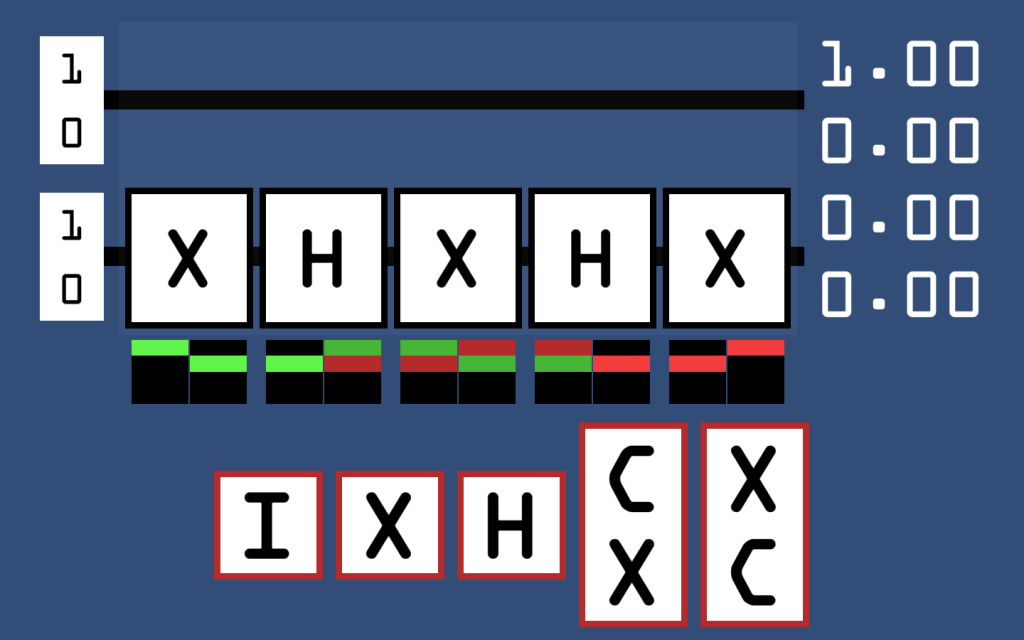
You probably also noticed the colours underneath the gate; they represent the actual values within the superposition as a colour, where green denotes a positive value and red negative. Black means a value of 0, and duller shades correspond to smaller magnitudes of values.

Now try resetting the circuit and adding a CNOT (denoted by C and X) and recreating some of the states in the .gif at the end of the last section. You can also try using the upside down CNOT which effectively swaps the roles of its two inputs. Everything should be relatively straightforward so far, but here’s where things get interesting: try adding a H gate before the C in a CNOT like this:

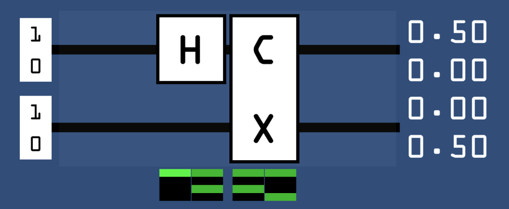
*Quantum entanglement, before your very eyes!*

Think about this output state for a second. Revisiting our coin metaphor, this represents a 50% chance for both coins to land on heads and 50% for both to land on tails – the coins can never land on opposite sides! They are inextricably linked to always be synchronised, no matter what side they eventually choose to land on, and even no matter how far apart they are physically separated. You may be thinking that the 2 coins are simply deciding on which side to land on ahead of time, but there exist situations that prove this is impossible (I will not go into detail on these so called Bell inequalities here, but a fun example is known as the CHSH game). This result has been rigorously tested through experiment, with a current world record distance of over 1000km, performed onboard satellites in outer space! This is amazing, but is also the reason why we cannot use two circular state machines to visualise the state anymore, because this superposition cannot ever constructed from a tensor product (FOIL) of 2 input qubits. Try it yourself and you’ll find that it’s mathematically impossible.

This fact reveals the reasoning behind the name entanglement, as the states of the individual qubits are now literally inseparable. Unfortunately it seems as if we now need a four dimensional diagram to construct an ideal representation of all possible superpositions of 2 qubits. This is why I mentioned earlier that I do not like the intuition of the upper qubit ‘controlling’ the other, because the two cannot even be treated separately in cases like this. What’s worse, the situation gets exponentially more complex with each additional qubit! But we’re getting ahead of ourselves; let’s use the tools we currently understand to solve an actual problem.

The Deutsch Oracle

We now know (almost) everything we need to know to solve a simple, if a little contrived, problem. Let me set the scene – you are given a black box which performs one of the four classical single-bit operations. These are: do nothing so that input=output, negate the bit so 0->1 and 1->0, always set to 0 no matter the input, and always set to 1. These can be seen in the following graphic:

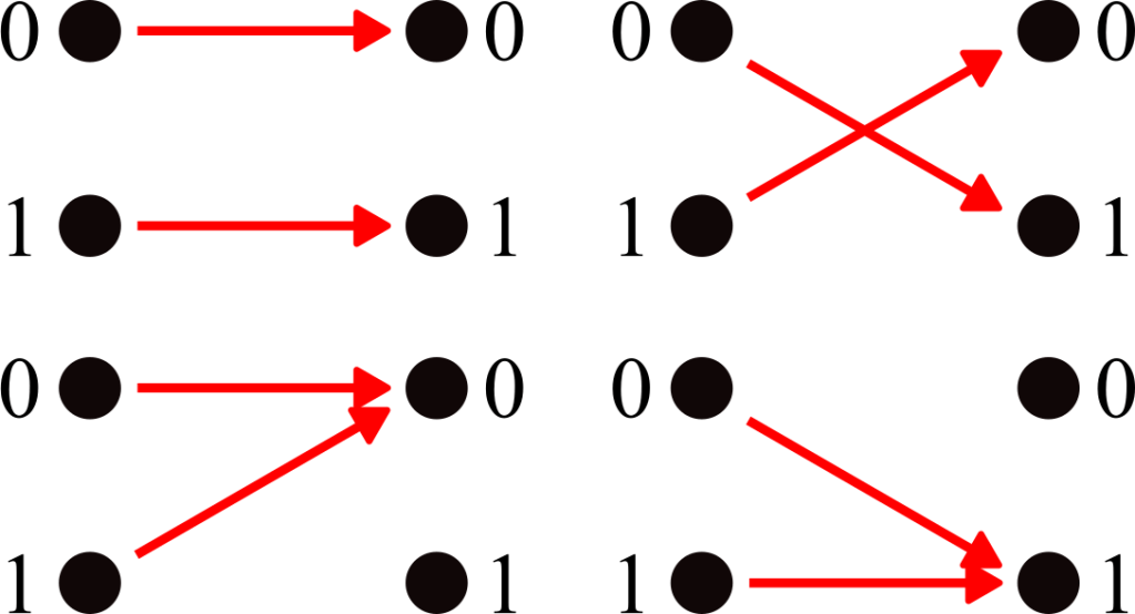
The four single bit operations. The top two are known as identity and negation, and the bottom two are constant-0 and constant-1.

Your task is simple: determine whether the output of the box is variable (one of the top two in the above diagram) or constant. However, it will shatter into a million pieces as soon as it is used once! This is impossible on a classical computer, as there is no way of differentiating the two groups without inputting both 0 and 1 into the box. We must therefore devise a clever strategy that only shoots one input into the box, leveraging the tools available to us only in the quantum world. But before we dive into trying to solve this, we must first construct the actual black box, which is surprisingly not trivial.

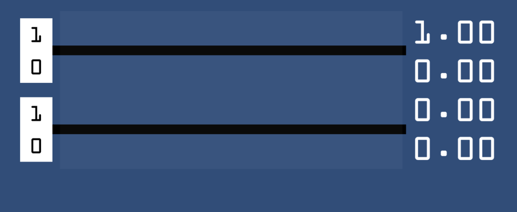
In the context of our quantum circuit, a classical bit=0 is equivalent to a qubit= $\begin{pmatrix}1\\0\end{pmatrix}$ , and bit=1 is qubit= $\begin{pmatrix}0\\1\end{pmatrix}$ . If you are very attentive you may have noticed that we cannot create the effect of the two constant functions using only X and H gates. Try it yourself on the simulator if you do not believe me. We must find another way to construct our black box, using one last trick that is important in the world of quantum computation: the concept of ‘ancilla’ qubits. I think the best way to explain this trick is to simply show you. This is what our constant-0 black box looks like:

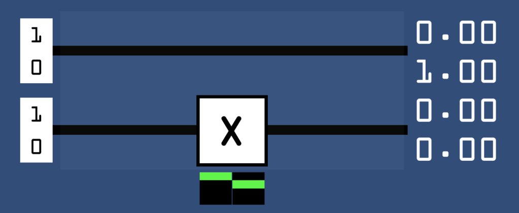
No, that is not the wrong image; it is simply an empty circuit! The trick here is that the upper qubit is our input, but the final value of lower qubit is our output. Additionally, the output value of the upper qubit will simply remain unchanged as it passes through, and the input value of the lower qubit is always set to $\begin{pmatrix}1\\0\end{pmatrix}$ . You can therefore think of the input of the lower qubit as auxiliary, and so it is called an ‘ancilla’. It should now be simple to guess what constant-1 looks like:

It is simply the first circuit but with an X gate on the lower wire. The identity box is a little more tricky, and if you’ve been wondering why I ever introduced the CNOT gate, this is why:

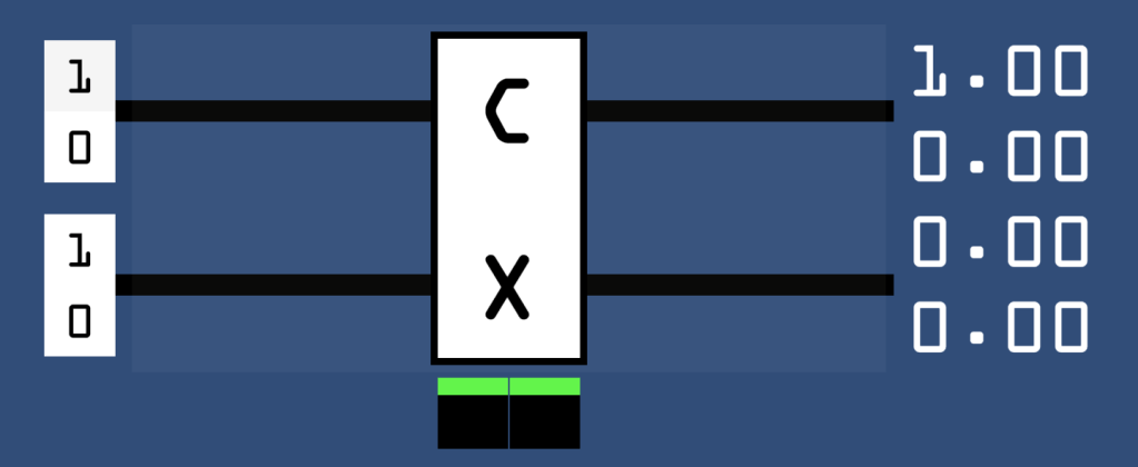
As you can see, our upper input qubit is now effectively controlling the outcome of the lower output qubit, and so they will always match each other at the output. The final possible black box is again similar:

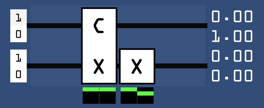
It is again simply the identity black box but with an X stuck on at the end. At this point it is worth noting that it is in fact not possible to construct a single qubit circuit that behaves like the constant-0 or constant-1 boxes, due to the fundamental laws of nature. Understanding why this is the case is out of scope for this post, but I will provide further resources at the end to give you a clue of where to look next.

You are now ready to try and construct a series of gates before and/or after these black boxes, that is able to determine whether its function is constant or variable with only one input. I’m not going to give you the answer! But I will strongly recommend one thing: forget about the numbers. The numbers (both on the far left and far right) will probably only be confusing because I haven’t explained their specifics in detail, so I want you to focus only on the colours that represent that state underneath the gates. See if you can make the colours stay equivalent when switching within categories, but change while switching between categories. And let me emphasise that red and green colours are equivalent in terms of the final result here.

I will also give you a couple of hints: try to emphasise the difference between the two categories, whilst suppressing the differences within each category. What do constant-0 and constant-1 have in common? And how do they differ from identity and negation? You may also find it useful to revisit the circular state machines in the earlier sections, to see if you can find configurations that allow you to emphasise or suppress certain gates. And here’s a spoiler if you’re struggling (highlight the next paragraphs if you want to see the steps):

The difference within groups is the X gate, while the difference between groups is the CNOT. How can we first nullify the effect of the X gate? In fact, all four non-deterministic positions (on the diagonal of the circular state) will nullify the X, because these four all produce the same result when measured. To nullify the X, we therefore place a H gate both before and after it, on the bottom wire.

Unfortunately only doing this makes all four black boxes produce the same output! So we need to add a couple of more gates to bring back the effect of the CNOT. The first step is to add an X before the bottom H, which introduces some red into the colours, but sadly the CNOT only affects the 3rd and 4th values so this doesn’t make a difference yet.

We therefore add another H gate onto the top wire before our black box, which ‘spreads’ the green and red into all four values in the superposition. This means that the CNOT will have an effect again!

The final step is to tidy up our output, as we need a deterministic output state to actually know the identity of the black box. We therefore add one more H gate onto the top wire, after the black box. You should notice that before this final gate, the output is split between the 2nd and 4th colours, which implies that only the top wire is non-deterministic. A final H gate on top ‘absorbs’ this back into a single state.

I do hope you enjoy playing with the simulator, and that it offers something a little different from the other introductions to quantum computing out there on the internet. If you get completely stuck then I’m sure you’ll be able to simply Google the answer ;).

Further Resources and Notes

The code for the simulator is openly available on GitHub.
The narrative of this post largely follows the one of a great talk given at Microsoft by Andrew Helwer. You can view it here.
The narrative of that talk also largely follows that of a paper written by Noson Yanovsky, from which the title of this post is also inspired. You can read it here.
A good university-level course (that is freely available online!) can be found at Carnegie Mellon University by Ryan O’Donnell. Lecture notes and accompanying recordings of said lectures can be found here.
The specific reason why we cannot recreate constant-0 or constant-1 on a single qubit is that gates are mathematically defined as matrices that multiply a given superposition. The X and H gates are therefore 2×2 matrices, and the CNOT is a 4×4 matrix. These matrices must be doubly stochastic, which means that the sum of each of its rows and each of its columns must add up to 1, and it is impossible to formulate such a matrix to always set a qubit to a constant value.
You may then wonder how the single-qubit X and H gates behave on superpositions that have 4 values, especially entangled ones. The answer to this is also in matrices: if you only have an X/H on one wire and the other is empty, we can treat the empty wire as a 2×2 identity matrix and then use the Kronecker product to construct the 4×4 matrix to apply to the overall superposition.
This information on matrices probably does not make any sense unless you see it written down, and I purposely left the extra maths out of the post to keep it high-level. However I am fully aware that leaving out specifics may have the effect of reducing clarity rather than improving simplicity, and if that is the case then I can only apologise and refer you to the resources above.
The values a qubit can take can not only be negative, but can also be complex! Luckily the state machine can still be visualised using what is known as a Bloch sphere.
You may also be wondering how qubits are actually implemented in the real world. This is a very modern area of research, and there are many possibilities that engineers all over the world are working on.
If you want to play with an honest-to-goodness real quantum computer, you can! IBM have made their own one available on a cloud service platform here. It also uses the quantum circuit model that I greatly simplified for the interactive simulation, so if you can use my simulator then you should be able to get to grips with the IBM one. If you do decide to try it however, do note that the symbol for the CNOT gate is different there.

As you dive deeper into the theory, you may (as I did, and still do) feel a little frustrated and lost in all the fancy technical language and mathematics. Unfortunately a more thorough knowledge of the underlying maths is necessary to form a deeper understanding of what is really going on, but I strongly believe that the first step to understanding is a solid intuition. I also believe that the best way to build such an intuition is through interactivity, as there is only so much one can learn by reading. This post is my little attempt to provide this for the concepts I have learnt so far, and my one hope is that you will come away with the belief that you yourself have the ability to understand quantum computing.